Online course with on-demand video and live Zoom meetings: Introduction to R using a protocol for conducting and presenting results of regression-type analyses
In this course, we will provide an introduction to R and at the same time explain how to conduct data exploration, apply (simple) linear regression models, communicate results, and also determine optimal sample size (using power analysis) in case you want to set up a new field study or experiment.
We will use a 10-step protocol based on Zuur and Ieno (2016). The protocol takes us from the organization of data (formulating relevant questions, visualizing data collection, data exploration, identifying dependency), through conducting analysis (presenting, fitting and validating the model) and presenting output (numerically and visually), to extending the model via simulation.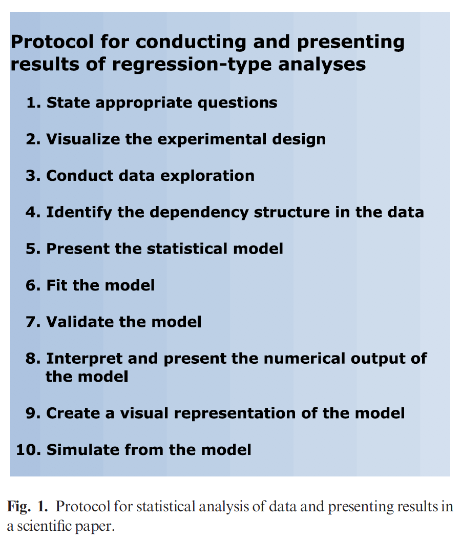
This course is for scientists who would like to learn R in a non-traditional approach by applying it in a playful way, and also for scientists who have been exposed to an introductory R course and would like to extend their skills to the next level. This course is also beneficial if you would like to learn data exploration, data visualization, apply linear regression models, and power analysis.
This online course contains various modules representing a total of approximately 10 hours of work. Each module consists of multiple video files with short theory presentations, followed by exercises using real data sets, and video files discussing the solutions. All video files are on-demand and can be watched online, as often as you want, at any time of the day, within a 6 month period.
A discussion board allows for daily interaction between instructors and participants. The course also contains a series of (approximately) 2-hour live web meetings in which we summarise some of the theory and exercises, and answer questions. Attending these live web meetings is optional. We will run the web meetings in different time zones.
Module 1
We will start this module with a theory presentation based on Zuur and Ieno (2015). Using a 10-step protocol, we will explain how to conduct a regression-type analysis and present the results. Note that we will not dive too deep into the statistical theory underlying the models.
We will then do 3 exercises that will teach you how to import data, manipulate data (deleting rows, selecting columns, etc), plot data using ggplot2, and formulate your questions as a preparation for the statistical analysis.
A more detailed outline is given in the two bullet points below.
- Introduction to R, theory presentation (10-step protocol), and executing steps 1 and 2 of the protocol in R. We will discuss the installation of R, R-Studio, and add-on packages, importing data into R and accessing variables.
- We will present various data sets and discuss how to formulate the underlying questions (which will motivate the application of certain statistical techniques). We will use the ggplot package in R to visualize spatial-temporal data and explain how to modify and manipulate data sets in R (e.g. removing rows or columns, creating new variables, etc.).
Web meeting 1: A 2-hour web-meeting will be scheduled. We will summarise module 1.
Module 2
In this module, we start with a theory presentation on data exploration (based on Zuur et al. 2010). We will apply data exploration on 3 data sets. We discuss how to recognize outliers and what to do with them. We also explain how to identify the presence of collinearity (correlation between covariates) using multipanel scatterplots, Pearson correlations, variance inflation factors, and principal component analysis biplots. All statistical techniques are explained in Laymen's terms. We also explain that you should not test the response variable for normality (which is a huge misconception).
The bullet points below summarise module 2.
- Conduct data exploration in R and visualize the dependency structure in the data (steps 3 and 4 of the protocol).
- We continue with the visualization of spatial data, time-series data, and spatial-temporal data. Data exploration is applied to various data sets using R functions like the plot, boxplot, and dotchart functions. However, the emphasis is on the ggplot2 package to make multipanel graphs.
Web meeting 2: A 2-hour web-meeting will be scheduled. We will summarise module 2.
Module 3
The third module consists of three exercises. In the first exercise, we execute a linear regression model with one covariate and apply the entire protocol. We explain how to apply the model, read the output, judge whether the model is good using model validation, and show how to visualize it using ggplot2. In the second exercise, we use a linear regression model with two covariates, and the same protocol is applied. Although we use a simple linear regression model, similar steps should be applied for more advanced models (e.g. linear mixed-effects models, GLMMs, or GAM(M)s).
In the third exercise, we use one of the data sets that we used earlier in the course. We ask the question: 'If we were to repeat the sampling process, how many observations should we take?' The statistical tool to answer this question is called 'power analysis', and it is surprisingly simple. We will use power analysis to determine what happens if we take fewer, or more observations. We will also investigate how many observations we need to take if we want to be able to detect a 20% change in the response variable, a 10% change, and a 5% change. A power analysis can save you a lot of money and time! We will program the power analysis from scratch. Power analysis can also be applied to more advanced models like GLMM (although that is not part of this course)
The bullet points below summarise the third module.
- Two exercises in which we apply steps 5 - 10 of the protocol.
- We assume that you are familiar with the basics of linear regression (a Laymen's explanation is provided). We will show how to implement such a model in R, explain how to assess the underlying assumptions, and visualize the model.
- We will also explain what to present in a paper or report.
- One exercise explaining and applying power analysis to determine the optimal sample size.
Web meeting 3: A 2-hour web-meeting will be scheduled. We will summarise module 3.
Web meetings: Web meetings are hosted on zoom.us. Click here for recommended internet speed (see the text under 'Recommended bandwidth for Webinar Attendees'). We will record the meetings and make them available on the course website.
Discussion Board: You can use the Discussion Board to ask any questions related to the course material.
Pre-required knowledge: Basic statistics (e.g. mean, variance, normality). No R knowledge is required. You will learn R ‘on the fly’. This is a non-technical course.
Cancellation policy: What if you are not able to participate? Once participants are given access to course exercises with R solution codes, pdf files of certain book chapters, pdf files of PowerPoint or Prezi presentations, and video solution files, all course fees are non-refundable and non-transferable to another participant.
Copyright: Sharing the access details of the course website or the pdf files of our course material is prohibited. Video files cannot be downloaded, but they can be watched in the same way as on Netflix.